Quantifying Spatial Audio Quality Impairment

Spatial audio quality is a highly multifaceted concept (see this for a very long list of things to consider). “Geometrical” components of spatial audio quality are perhaps the least subjective aspect of spatial audio quality to quantify, yet there have been very little attempt at dealing with it since BSS Eval came out almost 20(!) years ago.

Even the geometrical component of spatial audio quality is not trivial to quantify. We resorted to only considering the interchannel time differences (ITD) and interchannel level differences (ILD) of the test signal relative to a reference signal. With this, it is actually possible to construct a signal model to isolate some of the spatial distortion. By using a combination of Weiner-style least-square optimization and good ol’ correlation maximization, we propose a signal decomposition method to isolate the spatial error, in terms of interchannel gain leakages and changes in relative delays, from a processed signal. These intermediates parameters can then be used as a diagnostic tool to identify the nature of the spatial distortion and to quantify the spatial quality impairment.

Our work is open-sourced here both as a Python package and a CLI.

Warning: There’s a lot of math in this section. I’m sorry.

Methods

Let’s call the reference signal \(\mathbf{s}[n] \in \mathbb{R}^{C}\) and the test signal \(\hat{\mathbf{s}}[n] \in \mathbb{R}^{C}\). Here, \(C\) is the number of channels and \(n\) is the sample index. The signals might not be of the same length. That’s fine here.

We model the \(c\)th channel of the test signal as a sum of all the delayed and scaled channels of the reference signal, plus some other residual noise:

\[\hat{s}_c[n] = \underbrace{\sum_{d=1:C} A_{cd} s_d[n - \tau_{cd}]}_{:= \tilde{s}_c[n]} + \mathbf{e}_{\text{resid}}\]

We can interpret \(A_{cd}\) as the gain mapping from the \(d\)th channel of the reference signal to the \(c\)th channel of the test signal, and \((\mathbf{T})_{cd} = \tau_{cd}\) as the delay mapping from the \(d\)th channel of the reference signal to the \(c\)th channel of the test signal. Ideally, we want \(A_{cc} = 1\) and \(\tau_{cc} = 0\) for all \(c\), and \(A_{cd} = 0\) for all \(d \neq c\). The term \(\tilde{\mathbf{s}}\) is effectively the spatially distorted version of the clean signal, with no other types of distortion. We cannot actually guarantee that \(e_{\text{resid}}\) will contain no spatially relevant distortions, though. (If anyone has an idea on how to fix this, drop us an email!)

Objective Function

Now that we have a model for the spatial distortion, we can define an objective function to minimize the residual noise. Basically, we want to find the gain and delay mappings that minimize the difference between the test signal and the spatially distorted reference signal. This is done by minimizing the mean squared error between the test signal and the spatially distorted reference signal:

\[\min_{\mathbf{A}, \mathbf{T}} \sum_{\text{valid}\ n} \left\| \hat{\mathbf{s}}[n] - \tilde{\mathbf{s}}[n] \right\|_2^2\]

Optimization

Step 1

Finding the optimal gain is simple, but finding the optimal delay is not. So in practice, we could not easily do a joint optimization due to the non-convex nature of the objective function with respect to \(\mathbf{T}\). So we resorted to a very simple correlation maximization.

\[\tau_{cd} = \underset{-K \le \kappa \le K}{\operatorname{arg\ max}} \left| \underset{f \in \mathfrak{F}}{\mathrm{IDFT}}\left\{ \hat{S}_c[f] \cdot S^\ast_d[f] \cdot |H[f]|^2\right\}[\kappa] \right|\]

where \(H\) is an optional low-pass filter if your test signal is too noisy in the high end and \(K\) limits the search space.

Step 2

Once we have the optimal delay, we can find the optimal gain by solving a simple least-square optimization problem. This is very similar to the solution to the Wiener filter. The only differences are that (1) instead of computing an \(N\)-tap filter, we are computing a filter with no regards to the length, as long as there is only one non-zero tap at time \(\tau_{cd}\) with magnitude \(A_{cd}\); and (2) the filter is solved channel by channel.

Now, we form the autocorrelation tensor \(\mathbf{R} \in \mathbb{R}^{C \times (C \times C)}\) and the cross-correlation matrix \(\check{\mathbf{R}} \in \mathbb{R}^{C \times C}\).

\[(\mathbf{R}^c)_{bd} = \sum_{n} s_b[n - \tau_{cb}]s_d[n-\tau_{cd}]\] \[(\check{\mathbf{R}})_{cd} = \sum_{n} \hat{s}_c[n]s_d[n-\tau_{cd}]\]

Step 2.1

In (very) multichannel audio, sometimes we have silent channels. This makes parameter estimation very unstable. Like all problems in life, we pretend it’s not there and proceed.

\[\mathfrak{C}^{\perp} := \left\{c \in 1:C \mid \textstyle\sum_n |s_c[n]|^2 < \epsilon\right\}\] \[\mathfrak{D}^{\perp} := \left\{d \in 1:C \mid \textstyle\sum_n |\hat{s}_d[n]|^2 < \epsilon\right\}\] \[\mathbf{A}_{\mathfrak{C}^{\perp}, :} \gets \mathbf{0},\quad \mathbf{A}_{:, \mathfrak{D}^{\perp}} \gets \mathbf{0}\]

Step 3

Now, we can do the highly anticipated matrix inversion.

\[\mathbf{A}_{c,\mathfrak{D}} = \check{\mathbf{R}}_{c, \mathfrak{D}}\left(\mathbf{R}^{c}_{\mathfrak{D},\mathfrak{D}}\right)^{-1}\]

It’s a lot less math from here.

Error Decomposition

Let’s recap a little. We have

\[\hat{\mathbf{s}} = \tilde{\mathbf{s}} + \mathbf{e}_{\text{resid}}\]

but \(\tilde{\mathbf{s}}\) itself can be written as \(\tilde{\mathbf{s}} = \mathbf{s} + \mathbf{e}_{\text{spat}}\) where \(\mathbf{e}_{\text{spat}}\) is the noise that we know is definitely spatially related. Additive decomposition is not always the best way to do this, but it’s the easiest to understand. Let’s stick with this for now.

Now, we have two types of errors: the residual error and the spatial error. This now allow us to do what the source image to spatial distortion ratio (ISR) from BSS Eval originally set out to do. With this, we have the SNR-style metrics for spatial distortion, Signal to Spatial Distortion Ratio (SSR):

\[\text{SSR}(\hat{\mathbf{s}}; \mathbf{s}) = 10 \log_{10} \dfrac{\|\mathbf{s}\|^2}{\|\mathbf{e}_\text{spat}\|^2}\]

This measures the “amount” of spatial distortion in the signal, regardless of how much other types of distortion there are in the test signal.

The SSR also comes with a cousin, the Signal to Residual Distortion Ratio (SRR):

\[\text{SRR}(\hat{\mathbf{s}}; \mathbf{s}) = 10 \log_{10} \dfrac{\|\tilde{\mathbf{s}}\|^2}{\|\mathbf{e}_\text{resid}\|^2}\]

This measures the “amount” of residual distortion in the signal, regardless of how much spatial distortion there are in the test signal.

Some Benchmarks

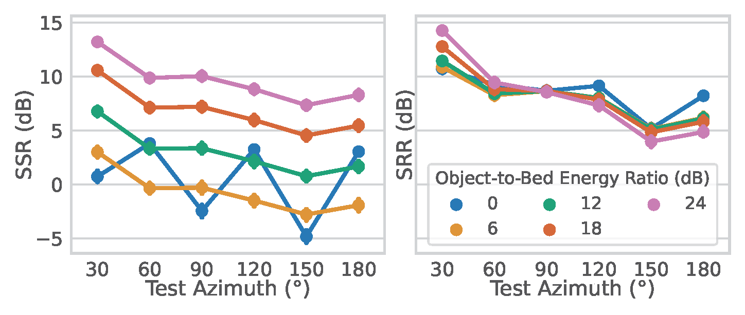
Although this work is designed to be a purely objective (instead of perceptual) tool, in that the main contribution is in the estimation of \(\mathbf{A}\) and \(\mathbf{T}\), we still need to verify that the SSR and SRR has the properties of (1) being robust to non-spatial distortion and (2) follows some perceptual intuition for well-established understanding of spatial audio quality.

Robustness Benchmark

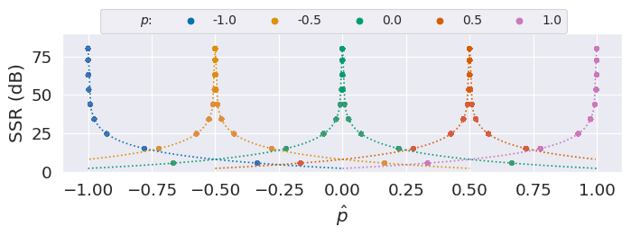
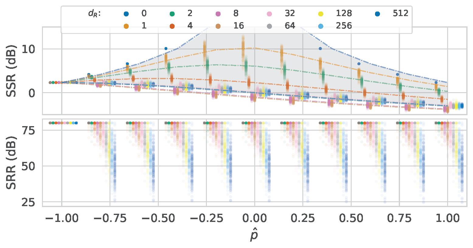
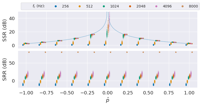
For this we stereoify the well-known Speech dataset TIMIT and test the metrics against panning, delay, filtering, and noise.

Panning only

Panning and delay

Panning and low-pass filter

Panning and noise

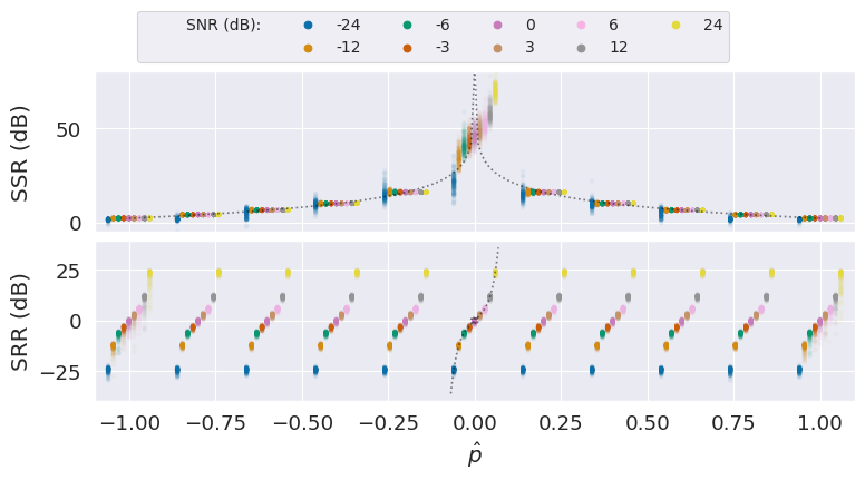
We also test the system by using the SPARTA to spatialize TIMIT and STARSS22 to 5 channels. For those with theoretical values, you will also see dotted lines in the figure below.

Codec Benchmark

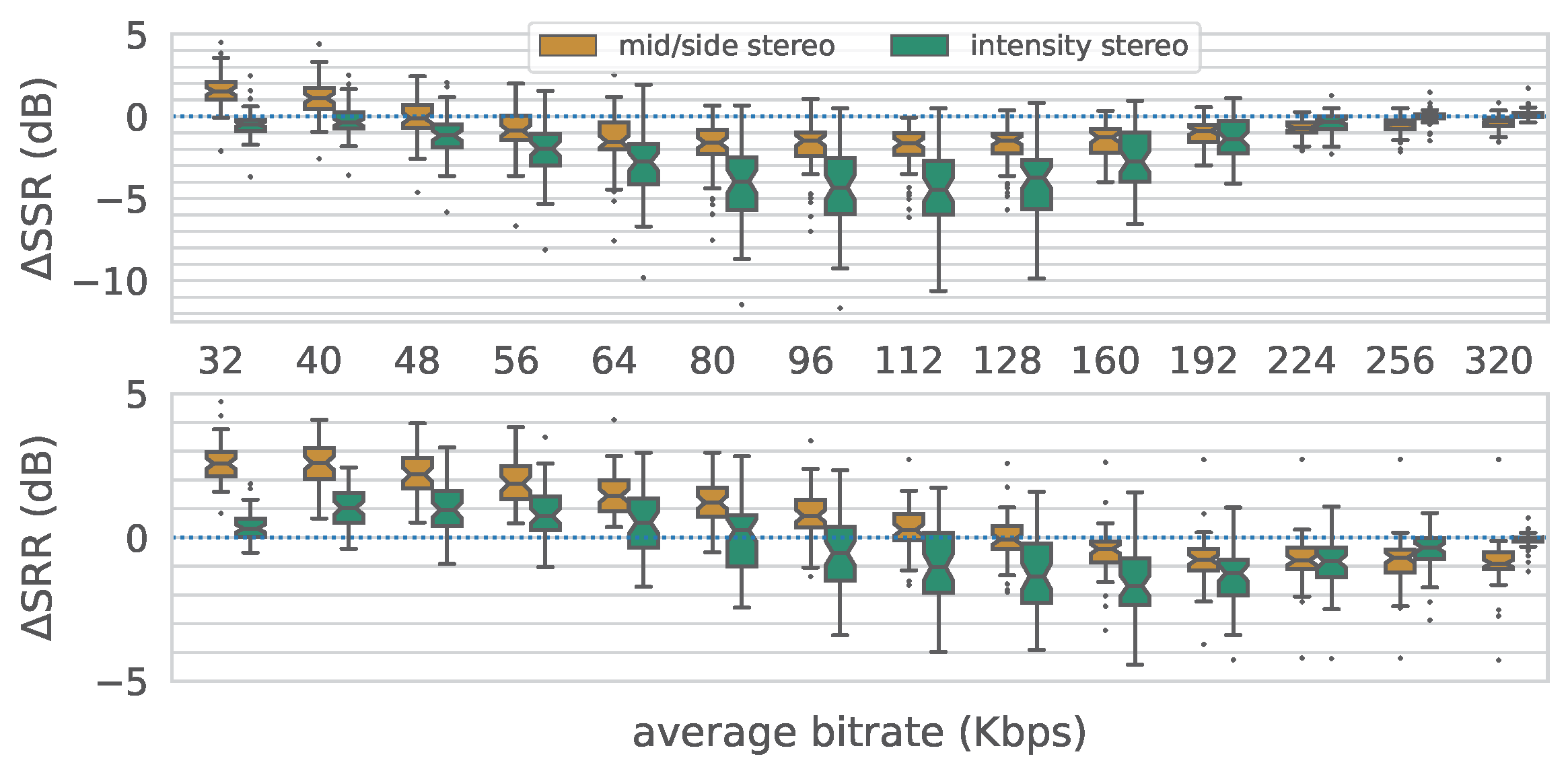
For this we use MUSDB18-HQ and compressed it using AAC under different stereo coding settings and test the compressed signals against the original.

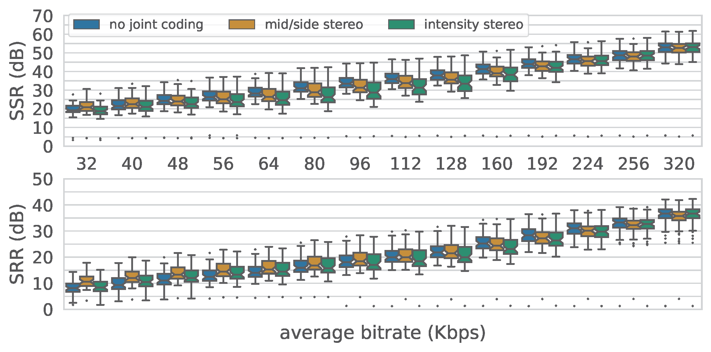
This figure is the same results as the above but we replotted-it to show the relative distortion instead of the absolute distortion. This clearly shows the tradeoff between using L/R, M/S, and joint coding as the bits are allocated between the content and the spatialization.

Conclusion

In this work, we propose a decomposition technique (that’s actually quite simple) to isolate the spatial distortion parameters, namely, the gain mapping and delay mapping matrices. Using these parameters, a number of downstream metrics can be proposed. We demonstrate two very simple energy-ratio metrics and benchmarked it against a number of spatial distortion scenarios.